THE VALUE OF 3D SEISMIC IN TODAY'S EXPLORATION ENVIRONMENT
-- IN CANADA AND AROUND THE WORLD

Cooper, N.M.1

1Mustagh Resources Ltd., Calgary, 400 604 -- 1st Street SW, Calgary, Alberta T2P 1M7, e:mail: ncooper@mustagh.com

OVERVIEW

Exploration for oil and gas involves the evaluation of a variety of information. Well logs provide detailed information at specific locations, usually an area less than one meter surrounding the well bore. We use our knowledge of formation signatures to recognize depositional environments and try to project this information between wells.

Reflection seismic methods can be used to create images of the geologic changes between wells. These images can help complete a picture of the subsurface that should enhance the ability of the explorationist to successfully select future well locations. Seismic is an effective tool as long as it provides meaningful and helpful images for the desired objectives. The seismic tool must provide a cost efficient alternative to additional drilling.

3D seismic has become a common exploration and production tool. This year, about 1200 3D programs will be recorded in Canada. In fact, Canadian geophysicists are internationally recognized as experts in the design, acquisition and processing of 3D seismic programs. 3D has also taken a strong hold on seismic operations in the United States. In every country where the author has consulted (18 countries on 6 continents), 3D techniques are either being used or are under serious consideration. The following map indicates the locations of some of the more intense onshore 3D activity. It is by no means a complete record of activity levels.

What is it about 3D that is making it such a popular tool? What determines the cost of 3D seismic and how does it compare to 2D?

REVIEW OF 2D SEISMIC

Reflection seismic is a method that allows us to image changes in the subsurface geology by inducing an acoustic wave from near the surface of the earth and listening for the echoes from deeper stratigraphic boundaries (much like ultra-sound is used to create pictures of unborn babies in their mother’s wombs).


2D seismic is recorded using straight lines of receivers crossing the surface of the earth. Acoustic energy is usually provided by the detonation of explosive charges or by large vibroseis trucks. The sound spreads out through the subsurface as a spherical wave front. Interfaces between different types of rocks will both reflect and transmit this wave front. The reflected signals return to the surface where they are observed by sensitive microphones known as geophones. The signals detected by these devices are recorded on magnetic tape and sent to data processors where they are adjusted and corrected for known distortions. The final processed data is displayed in a form known as "stacked" data.

COMPARISON OF 3D AND 2D METHODS

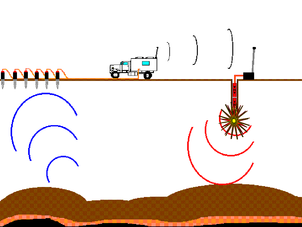
In the 3D seismic method, we record many lines of receivers across the earth’s surface. The area of receivers we record is known as a "patch". Often, we employ lines of source points laid out orthogonally to the receivers. By sequentially recording a group of shots lying between two receiver lines (referred to as a "salvo") and centered within the patch, we obtain uniform, one-fold reflection information from a subsurface area that is one quarter of the useful surface area of the patch. Although we usually record a large square or rectangular patch, the useful data at our zone of interest is offset limited by several geophysical factors. Therefore, we often consider the useful area of coverage as a circle with a radius equal to our maximum useful offset. By moving the patch and recording more salvos of source points, we accumulate overlapping subsurface coverage and build statistical repetition over each subsurface reflecting area (bin).

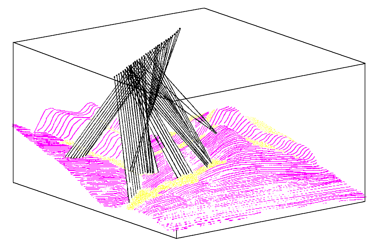
The quality of the sub-surface image obtained can be related to the statistical diversity of the information recorded for each cell of sub-surface coverage (known as a "bin"). The more observations obtained that contain unique measurements of the echoes from a certain area, the more successful we will be in re-constructing the subsurface geological configuration that caused those observations. The multiplicity (or "fold") of the recorded data for 2D and 3D methods is given by the following equations:

It is important to note that desired 2D image quality is controlled by our maximum useable offset (proportional to target depth) and governs our selection of source interval. 3D image quality is sensitive to offset squared and controls our selection of line grid density. The fact that 3D coverage is proportional to offset squared means that the economics of our program (grid density) and success of our program (image quality) are very sensitive to our evaluation of useable source-receiver offsets. We consider this factor to be of prime importance in a 3D design.

One of the most obvious differences between 2D and 3D seismic is that 3D imaging provides information continuously through the subsurface within the bounds of the survey whereas 2D seismic reveals only strips of information. Consider the images below and our ability to see both gross outlines and fine features when just a few lines are revealed versus a rough image of all points in the picture.


Now observe our increased ability to see distinct features (eyes, nose, lips, teeth, individual strands of hair) as the image quality is sharpened. If our objective is to see only the gross structural elements (where is the face ? ... Where is are the edges of the head ? ... Is the head separated from the shoulders ?), then the coarse image is sufficient and we need not spend the extra money to obtain finer image quality.

However, if the details of the structure are important, if a fault cuts across the structure (i.e. the thatch of hair crossing the face), then we need better image quality and must pay the price of better coverage. If we are pursuing subtle stratigraphic plays, we may need to see individual spaces within the fall of hair either side of the trace (analogous to sand bars within fluvial channels). Then we must attain optimal resolution and we will be concerned if the cost of the 3D still justifies the benefits we may achieve.


Furthermore, the final stacked data in 2D is plagued by source related noise, multiples, and incorrectly migrated events from out of the plane of seismic section (illustrated below in the picture on the left). To some extent, 3D methods improve each of these concerns. 3D imaging provides more traces and more diverse statistics to the seismic process. The picture on the right below shows three different recorded traces using three different source points and three different receiver points. All traces image the same mid point (where deep reflections are assumed to occur). Each trace represents a different source-receiver offset. Also, each trace represents a different source-receiver azimuth. Azimuth is a statistic unique to 3D recording and not a contributor to 2D processes. Azimuth adds a dimension of statistical diversity that is very helpful to the imaging procedure.


The magic of 3D is best conveyed by considering how we capture measurements of a returning wavefield. When we introduce acoustic energy in the earth, it is like dropping a large bag of ping-pong balls from the ceiling of a large room. The balls will bounce erratically from inhomogeneities in the room (chairs, desks, people). Many of the balls will return to the ceiling where their return could be observed and measured. By analyzing the timing and position of the returning balls, we can infer what irregularities may exist in the room. In oil and gas exploration, we are trying to image reservoirs and traps. Our image and reconstruction of the subsurface will be limited if we only receive the "ping pong balls" in distinct 2D lines. However, if we observe the reflected wavefield (ping-pong balls) over a large area, we will have much more useful information to construct our subsurface images.

Subsurface redundancy is determined by the density of source and receiver lines in proportion to the maximum useable source-receiver offset. Since shallow targets mean more restricted offsets, the density (and therefore the cost) of 3D programs for shallow objectives increases dramatically compared to surveys for deeper objectives. This phenomenon is not so noticeable in 2D since 2D parameters are not so sensitive to useable offsets.

Typical Costs of 2D Seismic

Play

Offset

Fold

Source

CDP

Cost

Type

(depth)

%

Interval

Size

(per km)

High Res

500

50

10

5

$7,500

Shallow

680

20

34

8.5

$6,500

Paleo U/C

960

12

80

10

$5,500

D-3

1400

14

100

12.5

$5,000

Deep

2000

20

100

12.5

$5,000

Foothills

4000

40

100

12.5

$30,000

Typical Costs of 3D Seismic

Play

Offset

Fold

Line

Bin

Cost

Type

(depth)

%

Spacing

Size

(per sq km)

High Res

500

20

100

5

$700,000

Shallow

700

10

200

15

$40,000

Paleo U/C

1000

14

240

20

$24,000

D-3

1400

18

290

25

$18,000

Deep

2000

20

400

30

$12,000

Foothills

4000

10

1120

40 x 100

$8,000

The above costs are approximate averages for the Western Canada Basin and should be used as guidelines for relative comparisons only. The "High Res" parameters refer to detailed 4D work performed of certain shallow enhanced recovery projects where the intent was to map advancing steam or fire fronts.

In order to record data with sufficient density over large areas, we require a large number of recording channels. The operations of 3D are considerably more elaborate than 2D and the daily cost of crew is substantially increased. However, the rewards include fewer dry holes, more optimized well locations, guidance for horizontal drilling projects, more complete evaluation of mineral rights and better understanding of the nature of prospects.

The following comparisons of 2D and 3D activities in Western Canada for the year of 1997 are compiled by personal communication with a sampling of clients, loose interpretation of industry statistics (total wells drilled from ERCB, crew activity levels from CAGC), and personal involvement in approximately 20% of seismic recorded in Canada. These interpretations do not represent any formal study or extensive surveys of the industry. None the less, we believe the following numbers represent the approximate state of the industry in a fairly accurate relative comparison.

2D versus 3D Seismic Activity Levels (1997)

2D

3D

Program Recorded


30,000 km

24,000 sq km
(1200 programs)

Crew Months

200

350

Channels per Crew

200

1200

Average Cost

$5,000

$350,000

Total Expenditure

$150,000,000

$420,000,000

2D versus 3D Estimated Results (1997)

2D

3D

Wells Drilled on Seismic


3000

8000

Drill Density

1 per 10 km

1 per 3 sq km

Seismic Costs /Well

$50,000

$52,500

Est. Completion Rate

60%

80%

Quality of Production

Fair

Good

Although 3D does not remove all exploration risk, it generally improves success rates and productive wells will more often be on optimal locations and should deliver better production and exhibit slightly longer life. One client who recently recorded a 3D over a well developed pool stated that six to ten of the dry holes associated with pool development would obviously not have been drilled if the 3D data was available prior to drilling. The costs of a 3D program may seem high, but the above figures indicate that exploration and development efficiency can be considerably enhanced by knowledgeable application of the 3D method.